

Decomposing Australian inflation
A standard Phillips curve decomposition framework to help monitor and understand movements in CPI inflation

By subscribing you’ll receive quality articles about the Australian economy and the world every month! Otherwise, liking or sharing is the best way to support my work. Thank you!
Australian CPI headline inflation has made a comeback from its dormant state. It has been below the RBA target range of 2-3% since 2014. However, the last CPI inflation was 5.1% over the year, the highest since 2001. This spike in inflation is not only hitting Australia but other countries around the world. High inflation has become a problem in most countries, but for different reasons. The Reserve Bank (Australia’s central bank) has started its tightening cycle by increasing the cash rate target to 0.85% and some expect it to be at 2.5% by the end of 2022. This has sparked much debate as to whether inflation is driven by external supply shocks, an overheating of the domestic economy, or both.
Understanding what is driving this recent increase in inflation helps us understand if fiscal and monetary policy should respond to mitigate these inflationary impacts on the economy. In this newsletter, I aim to explore this phenomena by using a simple framework to monitor inflation developed by Shapiro (2020) and replicate the methodology used in Sanders (2021) for Australia. This methodology is useful in understanding recent movements in CPI inflation.
The key assumption of this methodology is that inflation dynamics are best explained at the CPI component level. For each component, a standard Phillips curve model is estimated. A component is then labelled as either labour market-sensitive, exchange rate-sensitive, persistent acyclical or transitory acyclical based on the size and sign of a statistical value (t-statistic). This decomposition can help determine whether inflation is moving for reasons due to aggregate demand, or due to more specific factors such as external supply shocks. Fluctuations in aggregate demand, and consequently the economic cycle, directly impact inflation through firm’s price setting behaviour. This behaviour varies by sector, as some may be more sensitive to aggregate-demand conditions than others.
The labour market-sensitive inflation represents CPI components that have a significant relationship with labour market slack (the unemployment gap), while exchange rate-sensitive components have a significant response to changes in the Australian dollar (expressed by the import price deflator1). ‘Acyclical’ components do not have a statistically significant relationship with either the unemployment gap or the trade-weighted exchange rate. For instance, if the component’s inflation rate shows a negative and statistically significant relationship with the unemployment gap, the component is labelled as cyclical, otherwise it is labelled as acyclical. The acyclical components are further split into persistent — if it has a positive and statistically significant relationship with its past values — and transitory if not.
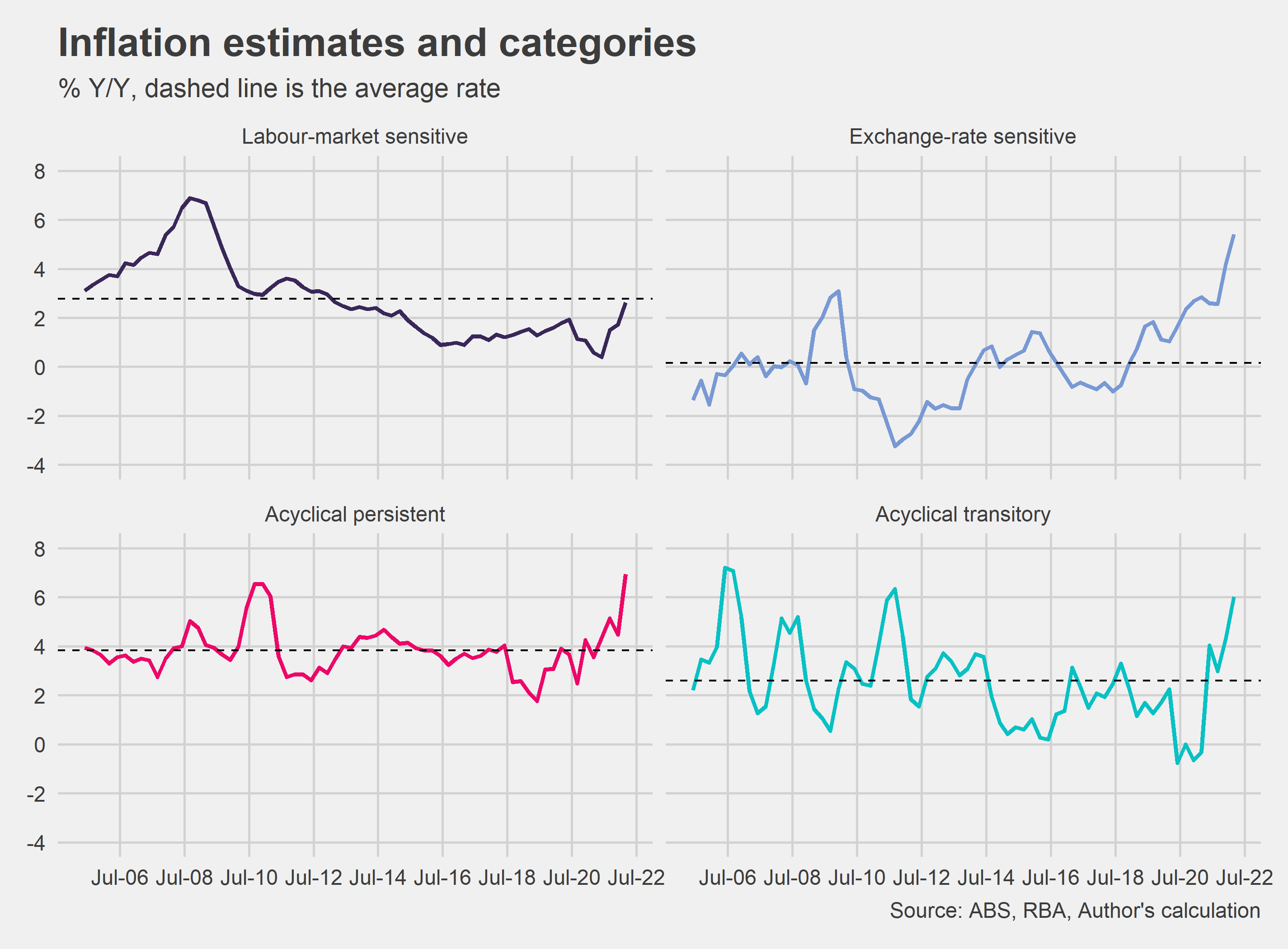
Figure 1 shows the decomposition of inflation into the four inflation estimated categories. We can see how recent developments in headline inflation have come from components that are sensitive to the import price deflator and acyclical to the domestic economy. The labour-sensitive estimate is still below its historical average rate but it is above its pre-Covid level, indicating that there is some heating in the domestic economy in recent quarters and may continue in the next few.
Labour-sensitive inflation
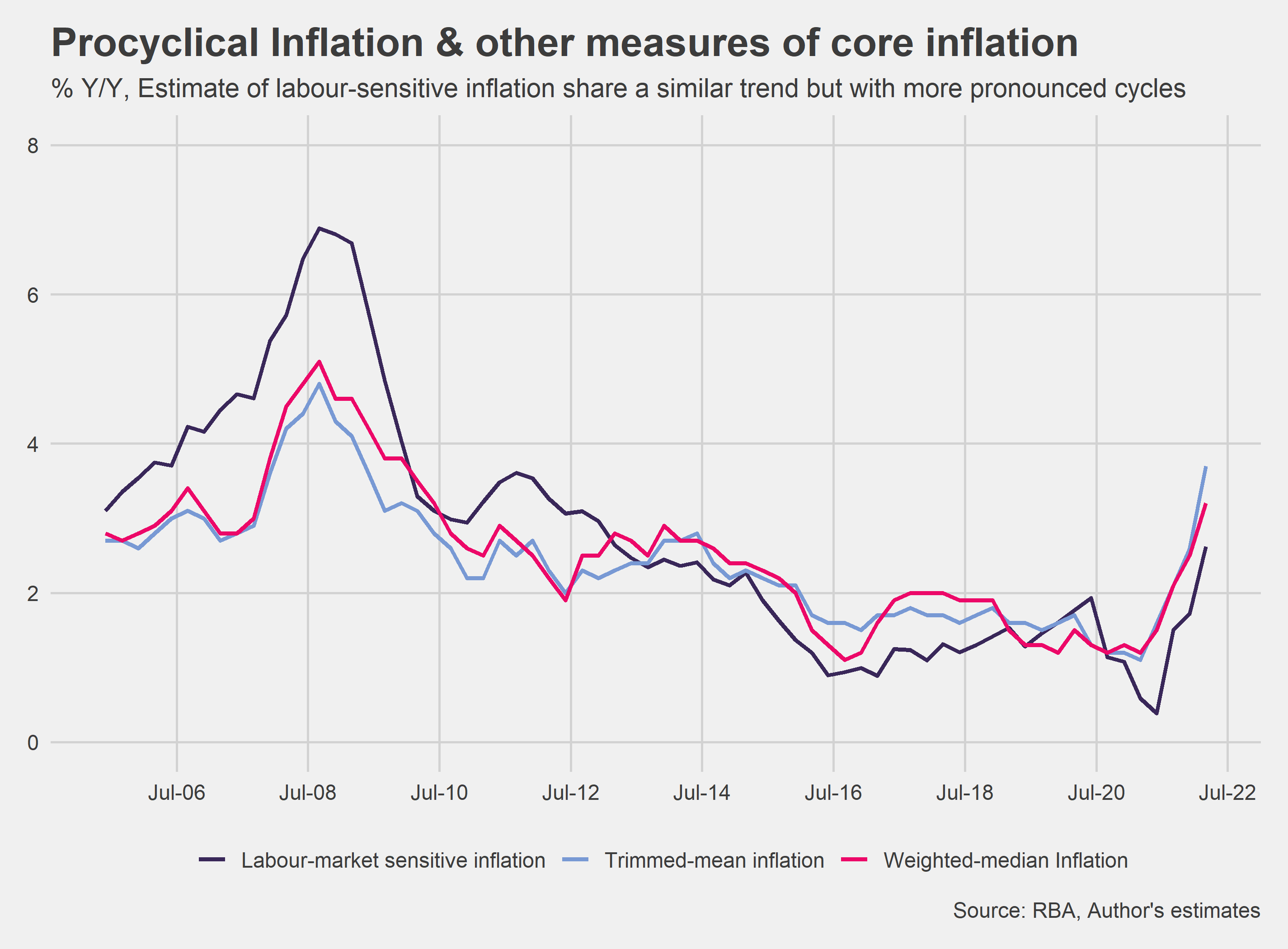
The labour-sensitive inflation estimated is of particular interest as it is a useful indicator of underlying cyclical inflationary pressures in the economy (it excludes volatile items and prices that have a weak relationship with domestic economic conditions). It should also isolate a key segment of the CPI basket that the Reserve Bank is aiming to affect when it sets monetary policy (with the ‘exchange rate-sensitive’ category being the other focal point). Moreover, Figure 2 shows that the estimate of labour-sensitive inflation has a similar trend to other measures of underlying inflation in Australia, but with more pronounced cycles. Labour market-sensitive inflation averaged 1.3% from 2015 to 2020 — compared to 3.8% in the decade prior to this. At its trough in 2016, annual labour-sensitive inflation was just 0.9%.
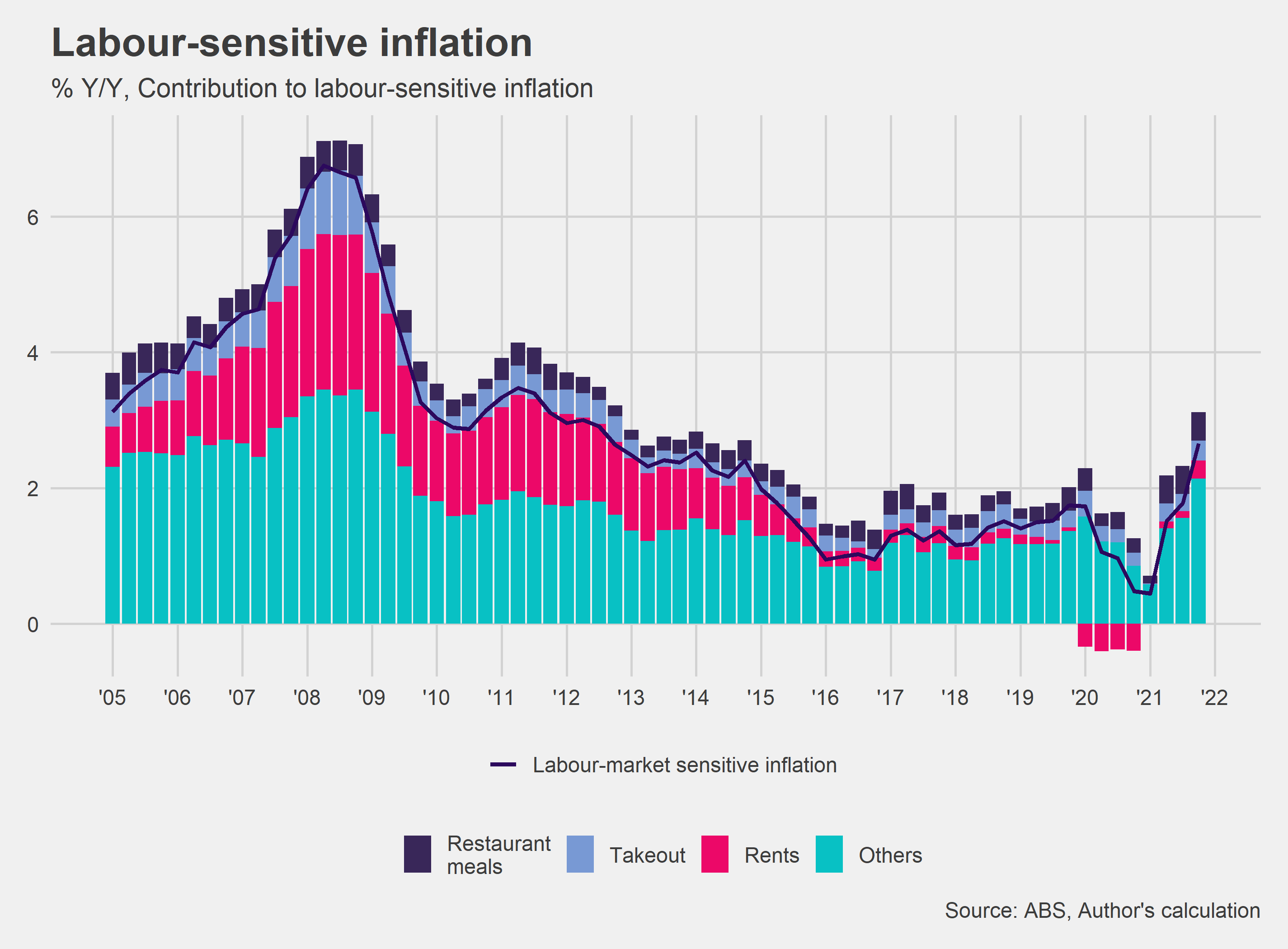
Additionally, this analysis suggests that the low level of inflation prior to 2021 is largely explained by a weak labour market (Figure 3). Rent inflation in particular has been a drag in the contributions to this category. Rent is a large component in CPI headline inflation (7%t of all household spending) and this is normally tied to the housing construction cycle. This also shows that the components sensitive to the economy cycle are not explaining the recent spike in headline inflation but they have started to pick up. Currently, vacancy rates are reasonably low and a substantial pipeline of dwelling supply is expected in the short-term. Therefore, it is expected we will see further increases in rent inflation (economist Zac Gross has a short thread about the rent component, which confirms this to be the case).
Exchange rate-sensitive inflation
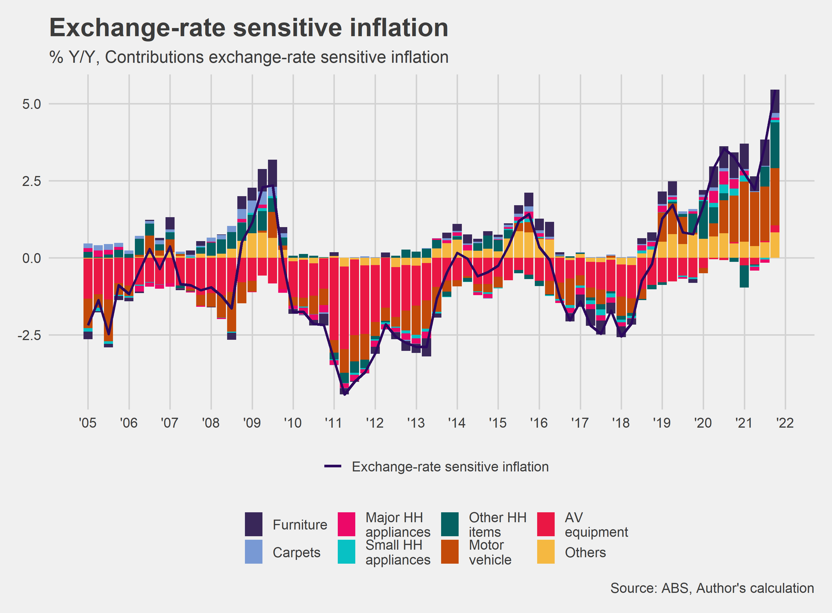
Contrary to labour-sensitive inflation, exchange rate-sensitive inflation has been above average in recent years (as seen in Figure 4). This pickup is larger than expected based on the depreciation of the exchange rate. Most of the components of the exchange-rate sensitive inflation are tradeable goods such as cars and appliances, which are items that are largely determined by world markets. The recent strength is possibly explained by disruptions to global supply chains mainly in China. The exchange rate will appreciate and cause a decrease in exports, if further increases in the cash rate continue, all things equal.
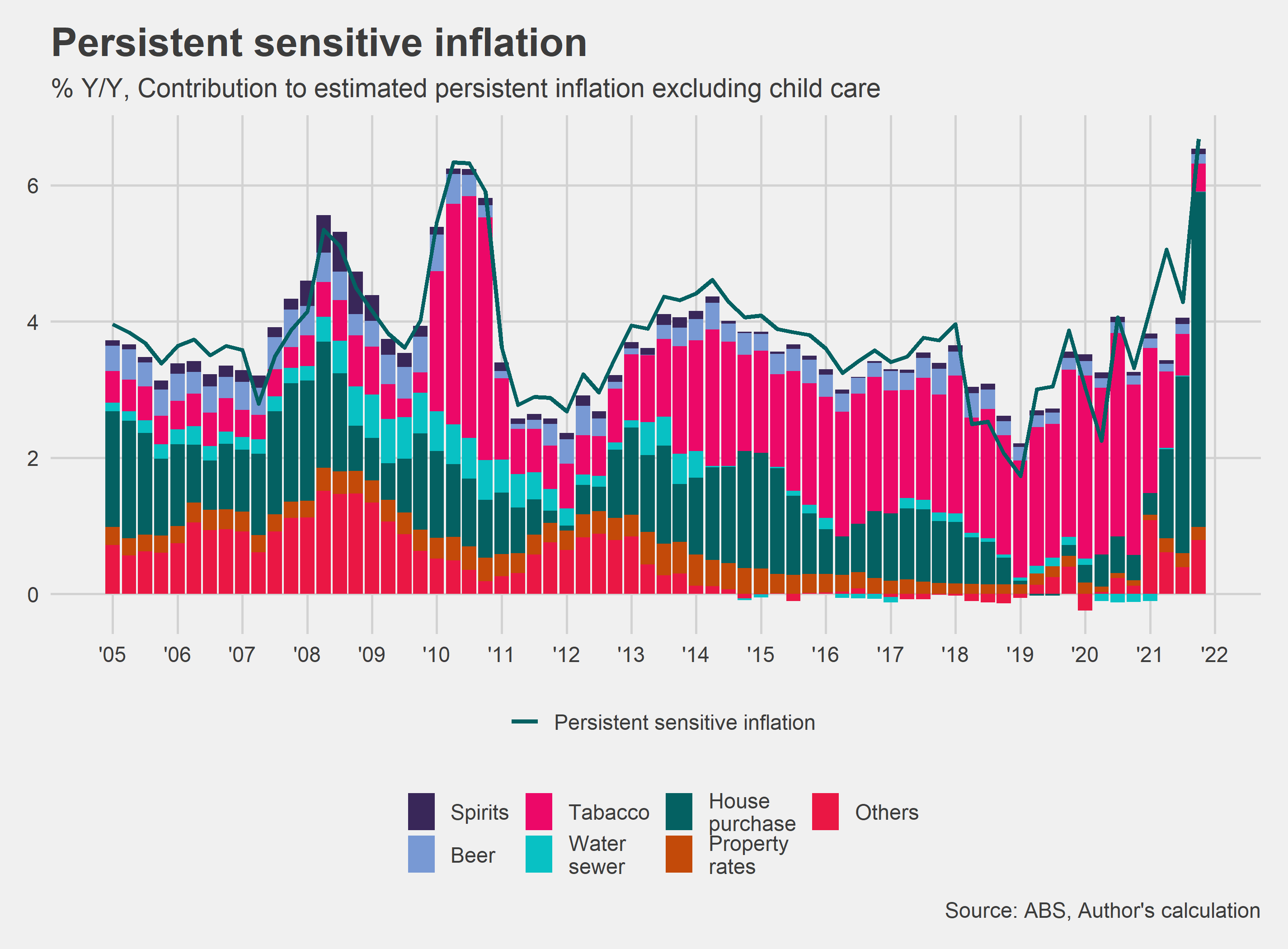
Persistent-sensitive inflation
Figure 5 shows the components that contribute to the estimate of persistent-sensitive inflation2. Most of the increase in persistent-sensitive inflation from 2010 to 2020 is due to the increase in tobacco excise implemented during that period. From mid 2021 the increase was due to house prices. We should expect to see further reductions in house prices and consequently in this inflation category, as the cash rate target increases going forward.
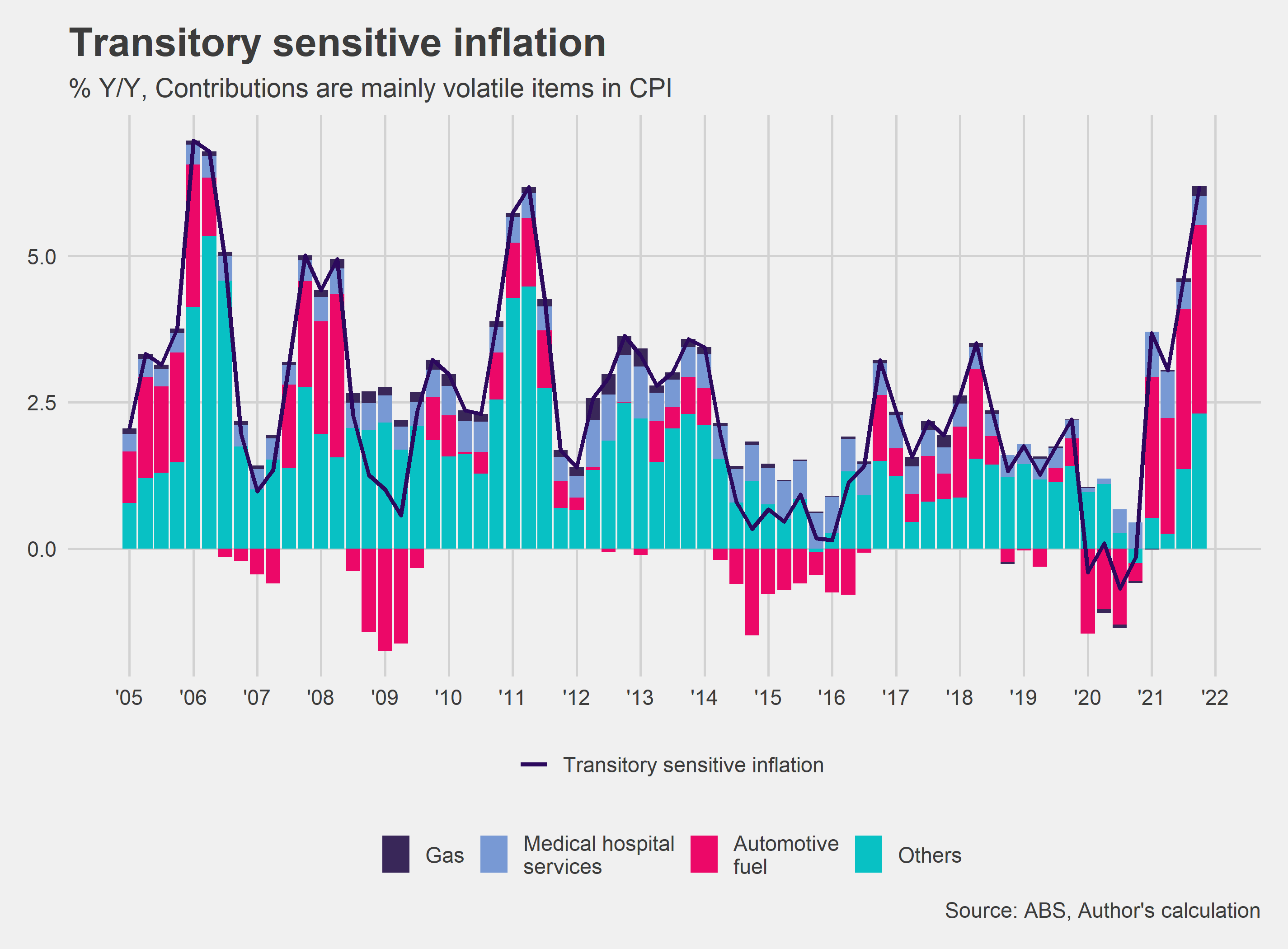
Transitory-sensitive inflation
Lastly, Figure 6 shows the components that contribute to the estimate of transitory-sensitive inflation. It is comprised of the most volatile items in CPI headline inflation. As we can see, fuel has been the main contributor since mid 2021, after the normalisation of economic activity in the country. This is not surprising to anyone who uses a car in Australia after seeing record highs in petrol prices at the bowser. Another volatile item that could follow suit is gas - if the domestic demand for gas is outstripped by the demand required in Europe, after banning Russian gas in that market. In this category, there is little monetary policy could do as these prices are set internationally.
Conclusion
The Australian inflation problem is a combination of two main stories. The first was a strong demand that originated from a historical amount of fiscal and monetary stimulus. This led to strong household consumption and a strong economic recovery with Gross Domestic Product above pre-Covid levels. However, it does not explain the strong inflation numbers. The second was the supply shocks created by the conflict in Europe and supply chain disruptions in China. These shocks led to an increase in imported prices in most of the tradable components in the CPI. All the categories of inflation shown in this article except labour-sensitive, are above its historical average. This tells us that our inflation problem is not mainly due to an overheating economy.
The RBA is right to normalise monetary conditions, but strong breaks in the still-in-recovery phase of the economy would not reduce the high levels of inflation in the short-term. Fiscal policymakers should step in to provide some relief to those at the lowest level of the household income distribution.
In this example, I use the import price deflator, but the traded-weighted exchange rate could also be used. The results do not change the allocation of the components in the inflation categories.
I excluded child care in this chart due to the base effect caused by the end of free child care in June 2021.